Experiments are a great way to measure what will change. To measure what has changed, (in absence of, or in addition to experiment results) we need a comparative analysis of the before vs after periods with respect to the sunset event, i.e., we need to conduct counterfactual analyses.
There are 2 approaches to apply counterfactual analysis for this scenario:
Notation: O(v) is observed values, E(v) is expected value.
- Testing for significant difference between the observed values: O(metrics pre-sunset) vs O(metrics post-sunset). In shorthand, O(pre) vs O(post).
This method is quicker but less robust. - Comparing expected value to observed values: E(metrics post-sunset) vs O(metrics post-sunset). In shorthand, E(post) vs O(post).
Here, E(v) are predicted to estimate a scenario where the sunset event never occurred. But, since the sunset event did occur, the difference of the E(v) from the O(v) explains the change after product sunset. This method is relatively more time-consuming but is also more robust.
Both approaches have their advantages and disadvantages.
| Approach 1: O(pre) vs O(post) | Approach 2: E(post) vs O(post) | |
|---|---|---|
| Feature selection1 |
Feature-agnostic: This method is suitable to be applied to a wide variety of metrics (or features) like, cross-sectional data (example: absolute count of active days per user), time-series data and pooled time series data (example: average or median active days across all users per month). | Time-series and pooled time-series only: Since this method involves predicting future values of a feature, this can only be done with time-series data or pooled time-series data (where a feature distribution is aggregated per time period). Furthermore, since no aggregate (average, median, etc.) is single-handedly representative of the complete distribution, selecting this approach involves the risk of losing useful information. |
| Robustness of results |
What this approach offers in breath of feature selection, it fails to offer in depth of robust findings. This can be compensated for by manually segmenting the data based on expected differentiators and, running significance tests for each segment (in addition to the whole distribution). However, the practicality of this is subject to the ease of proactively judging these segments from the dataset, and the increased risk of operating with confirmation bias. |
This approach of counterfactual analysis offers more depth of information to characterize significant differences between expected and observed results along a spectrum, rather than a single data point like in approach 1. One may, for instance, discover that not only is there significant difference but it occurs more in peak months of activity, compared to slump months of the product usage cycle. |
| Time investment |
This approach is relatively quicker to execute and, can be an optional first step to approach 2, to get a feel of the underlying dataset & patterns. | Fitting a time series model to each feature*, especially, for a new dataset, is usually more time consuming. |
1Here and onward, feature is used to mean variables/metrics in the data model (data science terminology), and not features of a product (product terminology).
Side note 1: Measuring change vs conducting causal inference
Note that the title of this paper reads ‘measuring the aftermath’ and not ‘measuring the impact’. The difference between the two is measuring change vs inferencing causality after product sunset. Let’s understand this better.
Measuring impact involves establishing a causal relationship between product sunset (cause) and the measured aftermath (effect). It seeks to answer the question that if there are significant differences in user behavior post-sunset, how much change is a result of product sunset vs other changes (marketing campaigns, new learning resources, etc.) or externalities (economic situation, new competitors, etc.). Measuring the aftermath (characterizing the effect) is a necessary pre-cursor to performing causal inference.
Causal modelling is a fascinating heuristic technique that involves several analytics techniques. Perhaps, this is why it is referred to as a mix of art and science. Much research is being done in this relatively new area and much is yet to be standardized, unlike our age-old techniques that have been smoothened and deepened, to cover not only the generic use cases but also niche variants. As is the current state, causal modeling application deserves its own paper and is out of scope here.
Approach 1: Comparing observed data pre & post sunset
Let’s take the example of 3 features to characterize product usage in the pre and post periods:
- Active users per month (MAU - a measure of user traffic),
- Median2 active days per user month (a measure of engagement),
- Days to first (replacement) product activity (a measure of adoption of the product replacing the one being sunset). Here, we assume that the replacement product is an existing product, i.e., it has usage data in the pre-sunset period.
2The choice of aggregate depends on the distribution of the cross-sectional metric. Most real-world adoption and engagement distributions tend to be heavily skewed and so, median is chosen here to represent the central tendency.
Let’s take a look at the feature types: MAU is a time-series feature, active days/month is a pooled time-series feature and, days to first product activity is a cross-sectional feature (unaggregated).
💡 Pooled time-series data is cross-sectional data aggregated per period to transform into time-series data. In approach 1, the treatment for time-series and pooled time-series features remain the same. The difference occurs in approach 2, when fitting a time-series model to predict future values.
Side note 2: Sample Period
Let’s assume 6 months of data per feature, immediately pre and post product sunset, for fair comparison.
Ideally, comparing annual data ensures a fairer comparison, i.e., lesser dependency on seasonality with respect to the months immediately pre and post sunset. However, since greater distance from the sunset event increases the risk of omitted influences (other explanatory variables not included in the feature set), this time horizon may not be acceptable to some use cases.
When we want to stay as close as feasible (with respect to the sample size) to the change event, this risk can be mitigated by decomposing the time-series features to remove their seasonal component (here onwards referred to as de-seasonalizing).
De-seasonalize time-series metrics
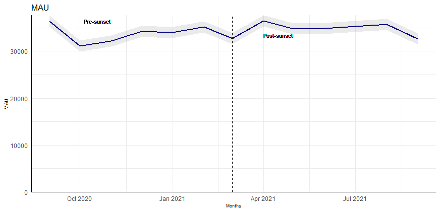
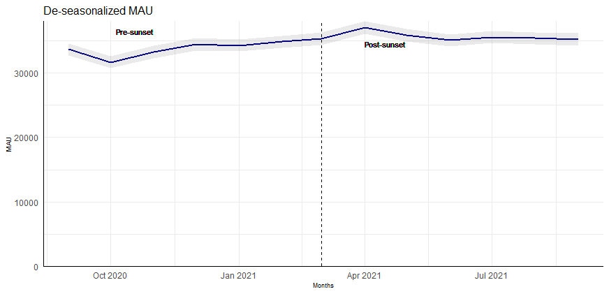
Here, we transform the MAU into a de-seasonalized MAU (see image 1) before testing for significant differences between O(pre) and O(post).


💡 Note: While sample period for pre and post comparison is 12 months (6 months each); for de-seasonalizing the time-series features, it is valuable to take as much historical data as available to aptly detect the seasonal component.
# code chunk for removing seasonality

# Sample data with seasonality
dates <- seq(as.Date("2020-09-01"), by = "month", length.out = 36) #sample dates
df <- as.data.frame(dates, col.names = "month") #dates added to data frame
df$sample_metric <- runif(n = 36, min = 10000, max = 30000) #sample metric data

#Create time series object
timeseries_data <- ts(df$sample_metric[order(df$month)],
                      frequency = 12,
                      start = c(2022,1))

#Decompose time series
timeseries_decomposed <- stl(timeseries_data, s.window = "periodic")

#Remove seasonal component
timeseries_deseasonalized <- seasadj(timeseries_decomposed)

#Add back de-seasonalized data to main df
deseasonalized.df <- data.frame(sample_metric_ds = as.matrix(timeseries_deseasonalized),
                                month = as.Date(time(timeseries_deseasonalized)))
df <- merge(df, deseasonalized.df,
            by = "month", all = FALSE)
Run Significance Test
The next important decision is choosing a suitable significance test to reject the null hypothesis of no change in the feature, that is, O(pre) = O(post).
This decision depends on several factors like, data type (numerical vs categorical), number of groups to be compared (pre vs post = 2 groups), relationship between groups (paired vs non-paired), sensitivity requirement of the effect (detect small vs large changes), etc. Our example includes only numerical features. These are then checked for normality, usually proven false in real world datasets, and applies the non-parametric Mann-Whitney U test. Other tests to consider are KS (Kolmogorov–Smirnov) test, AD (Anderson-Darling) test.
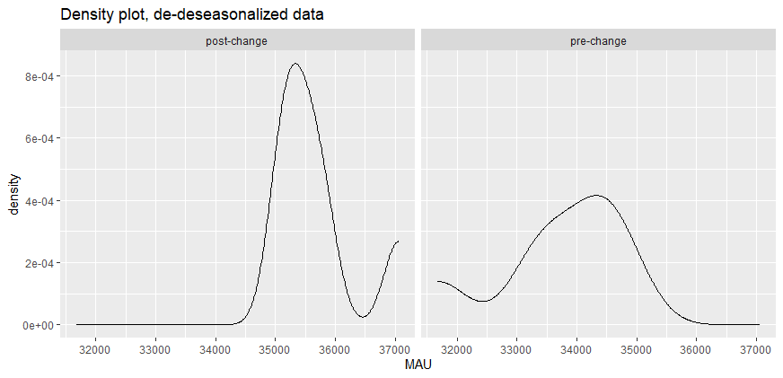
If there is a significant difference, we follow this by checking similarity of distribution (between the two groups), to correctly interpret the significance test results. In the density plot in image 2, we see that the distributions of the two groups of MAU are not similar and, hence, the change is interpreted in terms of mean rank difference. If the distributions were similar, we would interpret it in terms of the median.

# code chunk for running significance test + choosing the right interpretation
library(ggplot2)

#Continued from sample df created in previous code chunk
#randomly assigning months to pre vs post sunset periods
df$group <- c(rep("pre",18), rep("post",18))

#checking normality--------------------------------------/
#Alternative 1: Using a Q-Q plot
ggplot(df, aes(sample = sample_metric_ds)) +
  stat_qq() +
  stat_qq_line(col = "goldenrod") +
  theme_minimal() + theme(legend.position = "top") +
  facet_wrap(~group) +
  labs(title = "Normal Q-Q Plot", color = NULL)

#Alternative 2: Using Shapiro-Wilk test
shapiro.test(df$sample_metric_ds[df$group == "pre"])
shapiro.test(df$sample_metric_ds[df$group == "post"])
#note: the independent samples t-test is fairly robust to small deviations from normality.

#choosing significance test------------------------------/
# If the data is normally distributed & doesn't have outliers, use t-test.
# Else, use a suitable non-parametric test.
# Fro example, Mann Whitney U test:
pre <- df$sample_metric_ds[df$group == "pre"]
post <- df$sample_metric_ds[df$group == "post"]

#!!!Significantly increased from pre to post change on 99% confidence interval.
wilcox.test(pre, post, alternative = "less",
            exact = TRUE,
            correct = FALSE) #pre < post

#choosing the right interpretation of test results--------/
# comparing shape of data:
ggplot(df, aes(x = sample_metric_ds)) +
  geom_density() +
  facet_wrap(~group) +
  labs(title = "Density plot")

# If the shape is similar, the test results are interpreted in terms of the median. Else, the mean rank.

#calculating test stats for interpretation (wilcox.test() does not provide these automatically)
mw_test_manual <- df[, c("sample_metric_ds", "group")] %>%
  mutate(R = rank(sample_metric_ds)) %>%
  group_by(group) %>%
  summarize(.groups = "drop", n = n(), R = sum(R)) %>%
  pivot_wider(names_from = group, values_from = c(n, R)) %>%
  mutate(
    U_pre_change = `n_pre` * `n_post` + `n_pre`*(`n_pre` + 1)/2 - `R_pre`,
    U_the_change = `n_pre` * `n_post` + `n_post`*(`n_post` + 1)/2 - `R_post`,
    U = min(U_pre_change, U_the_change),
    m_U = `n_pre` * `n_post` / 2,
    s_U = sqrt((`n_pre` * `n_post` * (`n_pre` + `n_post` + 1)) / 12),
    z = (U - m_U) / s_U,
    mean_rank_pre_change = `R_pre` / `n_pre`,
    mean_rank_the_change = `R_post` / `n_post`,
  )
view(mw_test_manual)
These steps can be reapplied for pooled time-series features with an optional change: segmenting each group (pre and post values) for deeper insights.
For example, we may want to compare engagement separately for new vs existing users. In this case, the split is made before de-seasonalizing the pooled time-series, akin to splitting our original feature into two new features and analyzing each independently.
The steps followed for the cross-sectional features builds on the steps for time-series and pooled time-series features, with the exception of the de-seasonalizing step. The de-seasonalizing step may require further consideration depending on the nature of the chosen cross-sectional feature.
For example, values for duration-based features, like days to first activity, may exceed monthly bounds (a user can take 2 or 100 days within the sampling period). Here too, seasonality may play a role (a user may be slower during the Summer due to holidays or faster due to greater time availability) but this is deemed an indirect influence. Here, we have a trade-off to make between retaining information (comparing the full distribution) with the risk of indirect seasonality influence and, giving up information (aggregating cross-sectional data into pooled time-series data) to treat for seasonality. For such duration features, we may accept the risk of ignoring seasonal effect in favour of analyzing the full distribution.
While this trade-off cannot be avoided, its influence on the results can be minimized. One way to do this is by leveraging domain (industry/product) knowledge to segment the feature into 2 or more components: newer components transformed into a time-series feature (which is de-seasonalized and treated as afore-explained) and the remaining components stays a cross-sectional feature.
For example, if the sunset and replacement products are core offerings, we may see a high share of users performing the first product activity on their first day of interacting with our product ecosystem (i.e., median duration = 0). In this case, it may be beneficial to split our original feature, days to first activity on replacement product, into 2 new features: users with first activity on their first day (transformed into monthly counts over time, i.e., time-series data) and the rest of the distribution, i.e., where duration ≥ 1 day (remains as cross-sectional data).
💡 Note: Depending on the project needs, cross-sectional features can always be converted into pooled time-series features by choosing an aggregation. Partial conversion of cross-sectional data + de-seasonalizing choice depends on the feature context (like our reasoning for duration-based features) and the trade-off with information retention (analyzing a distribution vs an aggregate). For this context, the general recommendation is to always de-seasonalize time-series data where feasible.

